After writing the previous entry about Taleb and Mandelbrot I was thinking, “hey, I should be able to create the Mandelbrot set using R.” I’ve never actually tried to code the Mandelbrot set, but it seems easy enough. Well I messed with it for 2 maybe 3 seconds and then Googled [Mandelbrot set r] and, no surprise, I found a great implementation that not only produces the Mandelbrot set, it produces it with animation! As we all know, animation makes it betterer.

Pretty cool, ey? Well special credit goes to Jarek Tuszynski, PhD. over at Science Applications International Corporation who cobbled this together and posted it on a CRAN email list.
All the gory details (and source code!) after the break!
Here’s the R code Jarek wrote:
Z = 0 X = array(0, c(m,m,20)) for (k in 1:20) { Z = Z^2+C X[,,k] = exp(-abs(Z)) }
image(X[,,k], col=tim.colors(256)) # show final image in R write.gif(X, “Mandelbrot.gif”, col=tim.colors(256), delay=100)
Yeah, that’s it. It runs in 7.2 seconds on my laptop. It took me longer to find the gif on my harddrive than it did to run the code.
How’s it work, you ask? Freaking R magic, baby!
Oh, you want a real answer? Well, the logic works something like this:
Load up a couple of libraries solely for the creation of the animated gif and the colors:
Dr. T’ski likes to use the equal sign for assignment of variables. While I am sure he is a total R stud, this behavior is very ‘un-R.’ In my totally arrogant opinion he should be using the more common R syntax of ‘<-’ for assignment. So I would write the next bit like this:
to assign a value of 400 to the variable m
The next step he nests a bunch of stuff together and assigns that to the variable C. I’m going to break it up for explanation:
This creates a sequence of length 400 (since m=400) that ranges from -1.8 to 0.6. So that sequence looks a lot like this:
-1.800000000 -1.793984962 -1.787969925 … 0.587969925 0.593984962 0.600000000
except the ‘…’ is replaced by 394 values following that sequence.
The next bit sets the real property equal to a repeating pattern. (In this case he has to use the equal sign because he is not assigning a value to an object called[real], he is setting the real property of the [complex] function. Trust me. I used to be a Boy Scout)
This repeats each element of the previous sequence 400 times. So now the parameter [real] is set to a vector of length 160,000 that is the prior sequence, where each element is repeated 400 times. So that helps us understand the next part:
This is the sequence -1.2 to 1.2 in 400 steps where each step is repeated 400 times. It’s not the same as the previous step, but it rhymes. Now let’s bring that all together and define C:
since we already defined [real] and [imag] in the previous steps, let’s define C like this:
so C is created using the [complex] function on [real] and [imag] vectors. The [complex] function is looking for two parameters, real, and imag. Since we created two vectors by the same name, we used those. So if you try to run C <- complex( real, imag ) you get an error bitching at you about an invalid length.
So what, exactly, is C? It’s a complex vector made from the vectors [real] and [imag]. Not helpful? Well its a vector where each element has a real component and an imaginary component. So element number 1 of C (i.e. C[1]) is equal to “-1.8-1.2i”. Keep in mind that real[1]=-1.8 and imag[1]=-1.2. So C is a vector of length 160,000 where each element has a real component that comes from [real] and an imaginary component from [imag]. Head on over to Wikipedia if you need a refresher on complex numbers.
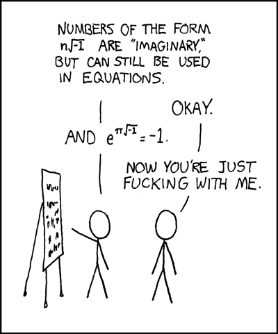
At this point you should be reminded of the following XKCD comic:
So now that we have that straight, what about the next bits? Well to good doctor T’ski now recycles the variable C to create a matrix using this syntax:
So [C] is now a matrix object of size 400 by 400. The [matrix] function just wraps the long vector C around so that the first 400 elements are the first row, the next 400 elements are the second row, etc. So now instead of C being a vector with 160,000 elements, it is a 400 by 400 matrix with 160,000 elements.
Now that we have C, let’s move on:
These two commands set up some objects that will bet populated later. [Z] is assigned a value of 0 and then X is created. X is a multidimensional array of size 400 by 400 by 20. So you can think of X as a 400 by 400 array where each element in that array is a vector of length 20. This is totally tangential, but in R you would access a given element using syntax like X[5,4,20] with the last element in the array being X[400,400,20]. Another way to think about X is to imagine a great big Rubik’s cube that instead of being 3 by 3 by 3 is of dimensions 400 by 400 by 20. Now picture looking at the 400 by 400 face of that big block. We are about to slice through each of the 20 layers. Oh yeah!
Everything up to this point is really just housekeeping to get ready for this next part that finally looks Mandelbrot-esque:
You’ll notice that this loop has 20 steps. If you’ll count the steps in the animated GIF above you will find that it, too, has 20 steps. Conicidence? I think NOT! Remember that 400 by 400 by 20 Rubik’s cube? (it’s really a hexahedron, not a cube, but stick with me) Each image in the animated GIF is a 400 by 400 layer from that big array. How does the loop work? I’m glad you asked!
The complex matrix we created earlier, [C] is going to be repeatedly squared and then have the original [C] added to it. If we refresh ourselves on the Mandelbrot Set we will remember (don’t you love how I assume we already knew this crap and just forgot it?) that the definition of the Mandelbrot set is a complex quadratic polynomial _z__n_+1 = _z__n_2 + _c _which remains unbounded. Well the loop above iterates through that polynomial.
The first time through this loop Z is 0 so Z^2+C ends up being just C. The next part of the loop takes the absolute value of each element in Z, then makes that negative. So all elements end up negative. Then the exponential function (exp) is applied to each element. So if the first two elements of Z had been 2,-3 they would be transformed into 0.135335,0.049787. The exponential function is required to transform the complex number into something that can actually be plotted. Look up at the cartoon above… see how you can raise e to the power of an imaginary number? Well the exponential function just raises e to the power of the each complex number in [Z]. Cool, ey?
From what I can tell it seems the ‘-abs’ bit is really optional. The image ends up the same if you simple do X[,,k] = exp(Z).
The whole matrix Z is then inserted as a layer into our 400 by 400 by 20 array. The very first layer (k=1) looks like this:

The next time through the loop (k=2) [Z] is much more complex. Instead of being 0, [Z] is now the initial matrix [C]. So on the second loop we square each element of [Z], add the elements of [C] to the squared values of [Z] then take the absolute value of each element, make each element negative, raise e to the power of each element (exponential function) and POOF we just created another layer of the image! We do that process 20 times.
The ‘real’ Mandelbrot set does not stop at 20 but rather continues for infinity. But the really neat thing about the Mandelbrot set is that as you iterate through the steps, the shape does not change… it just repeats the same pattern over and over and over at smaller intervals. It’s like zooming in to a beach from space. At first you see a rough shore line, then a rough rock, then bumps on that rock, then the roughness of the molecules that make up that rock. It just repeats as you zoom in. That’s fractals, Baby!
Author Clark hosted a great documentary on fractals titled “The Colors of Infinity.” Thanks to the interwebs you can watch the whole thing on YouTube!
Stay tuned, next week I’ll groom Schrodinger’s cat.
_ _